MySQL can do more than you think

In the last 13 years, I've used many programming languages, frameworks, tools, etc. One thing became clear: relational databases outlive every tech stack.

Let's understand them!

Building a database engine

Even better. What about building a database engine?

In fact, I've already done that. And wrote a book called Building a database engine.

You can already pre-order it if you want to support me 🙏

It's going to be available on the 8th of April. It discusses topics like:

• Storage layer
• Insert/Update/Delete/Select
• Write Ahead Log (WAL) and fault tolerancy
• B-Tree indexes
• Hash-based full-text indexes
• Page-level caching with LRU
• ...and more

Check it out and pre-order to get the best price:

In this article, we’re going to explore a few of its lesser known but very useful features. Things like Common Table Expressions, windows functions, partitions, and so on.

Common table expressions (CTE)

Take a look at this query:

select e.*
from employees e
join (
    select department
    from (
        select department, avg(salary) as avg_salary
        from employees
        group by department
    ) as dept_avg_salary
    where avg_salary > 75000
) as high_salary_depts
on e.department = high_salary_depts.department;

It has a subquery inside a subquery inside a join. It’s a bit hard to understand, right?

It returns employees that have a higher salary than department’s average they work in. Without knowing the context of the application, this is probably a good query if you consider performance. Another option is to get the average salaries for departments in one query, loop through the results, and query the employees in another query. It probably requires more memory and CPU and it’s going to be slower.

So is it a better way to write this query?

Yes, it is:

with 
    dept_avg_salary as (
        select department, avg(salary) as avg_salary 
        from employees 
        group by department
    ),
    high_salary_depts as (
        select department 
        from dept_avg_salary 
        where avg_salary > 75000
    )
select e.* 
from employees e
join high_salary_depts h on e.department = h.department;

This is called a Common table expression or CTE for short.

They provide a way to define named, temporary result sets that exist only within the scope of a single query. CTEs can make complex queries more readable and maintainable. Just compare these two queries.

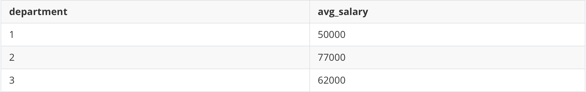
You can define a query with an alias that works like a table in the scope of the query. In this example, I create two “temp tables.” The first one stores the average salaries by departments:

dept_avg_salary as (
    select department, avg(salary) as avg_salary 
    from employees 
    group by department
),

You can think about this as a “temp table” with the following content:

In another CTE or in any part of the query it can be used as a normal table:

high_salary_depts as (
    select department 
    from dept_avg_salary 
    where avg_salary > 75000
)

And then high_salary_depts can be imagined as another “temp table” that contains only department IDs. It contains only one row with the ID of 2 in this specific example:

And then the rest of the query can use these CTEs as well:

select e.* 
from employees e
join high_salary_depts h on e.department = h.department;

It’s much easier to understand the query, and I think it’s closer to our thinking as well while writing these queries. It’s not a subquery inside a subquery inside a join. It’s an independent temporary table-like object.

CTEs are cool. But the next feature blew my mind.

Window functions

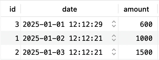
Given we have an orders table that looks like this:

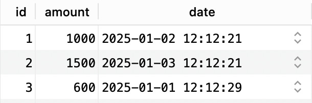
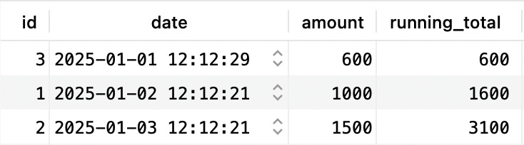
How would you query sales data with running total numbers? Something that looks like this:

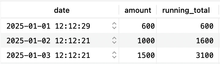
We often do these kinds of calculations in the backend code. But this can be done in a single SQL query:

select
    date,
    amount,
    sum(amount) over (order by date) as running_total
from orders;

This line is called a window function:

sum(amount) over (order by date) as running_total

Normally, sum() aggregates rows. Meaning, if you have 10 rows and you execute a sum() it returns one single row. Of course, you can return multiple rows using group by but the result will still be aggregated.

Window functions, on the other hand, do not aggregate rows to a single output row.

This expression:

sum(amount) over (order by date)

Reads like this:

sum(amount) → sum up the amount column over → over the following result set (order by date) → this is the result set. Take all rows and order them by the date column. The whole process can be imagined like this.

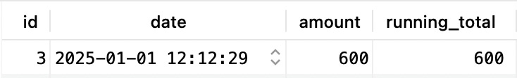
First, order the rows by the date column. The result now looks like this:

Then, iterate through the rows and for each one calculate sum(amount). So the DB engine starts with the first row, and calculates the sum for that single row:

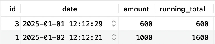
Then, it continues with the second row:

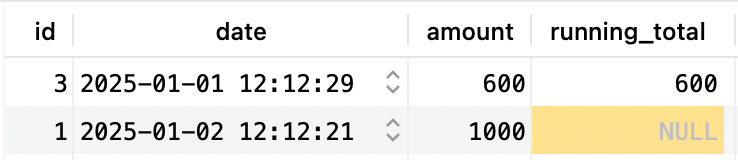
But this time, sum(amount) will actually result in 600+1000:

And finally, it continues with the third row, where sum(amount) will result in 600+1000+1500 giving us the final output:

Building a database engine

This whole article comes from my book - Building a database engine

It's going to be available on the 8th of April. It discusses topics like:

• Storage layer
• Insert/Update/Delete/Select
• Write Ahead Log (WAL) and fault tolerancy
• B-Tree indexes
• Hash-based full-text indexes
• Page-level caching with LRU
• ...and more

Check it out and pre-order to get the best price:

Partitioning in window functions

Given we have the same tables as before (an employee with a department ID and a salary) how would you write a query that returns this?

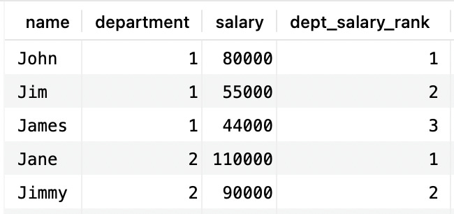
This is a list of employees grouped by departments, ordered by salaries, and each row has a rank number.

The query itself is quite easy:

select `name`, department, salary
from employees
group by department, `name`, salary
order by salary desc;

But what about the rank number? For that, we often write a function in the backend codebase. That works fine, but sometimes it requires too many iterations, too many memory consumption, etc. Once you reach a certain size it can become problematic.

The same result can be achieved without writing a single line of code, only a SQL query:

select 
    `name`,
    department,
    salary,
    rank() over (partition by `department` order by `salary` desc) as dept_salary_rank
from employees;

This query contains two new things:

• rank()
• partition by

There are multiple functions that can be used in windows operations. See the full list here. The rank() function is pretty simple. It assigns ranks based on the order by clause. If you have 5 rows ordered, the first one has a rank of 1 and the 5th one has a rank of 5. Easy.

partition by is very similar to group by. It is used to group together rows with the same column value. In this case, employees in the same department. After the grouping, window functions are then applied separately within each partition.

This is why the rank function starts over for a new department. It is executed separately for each group giving us a rank in a specific department.

Other interesting use cases for window functions:

• Moving averages with frame clause (using rows between)
• Running totals and cumulative sums
• Aggregate functions without aggregating the result set (sum, avg, count, min, max)
• Rankings and percentiles
• Time series analysis (things like year-over-year growth, etc)

I’m not saying this is the most easy-to-understand feature of MySQL, but there are cases when it will perform 10x compared to your PHP functions that run additional queries, load additional rows in memory, etc.

Partitioning

In the previous chapter, we talked about partitioning in the context of windows functions. The partitioning we’re going to talk about now is a different one.

As you might know, MySQL (and any other DB) stores your tables on the disk as a file. Usually, they’re located in /var/lib/mysql/<dbname>:

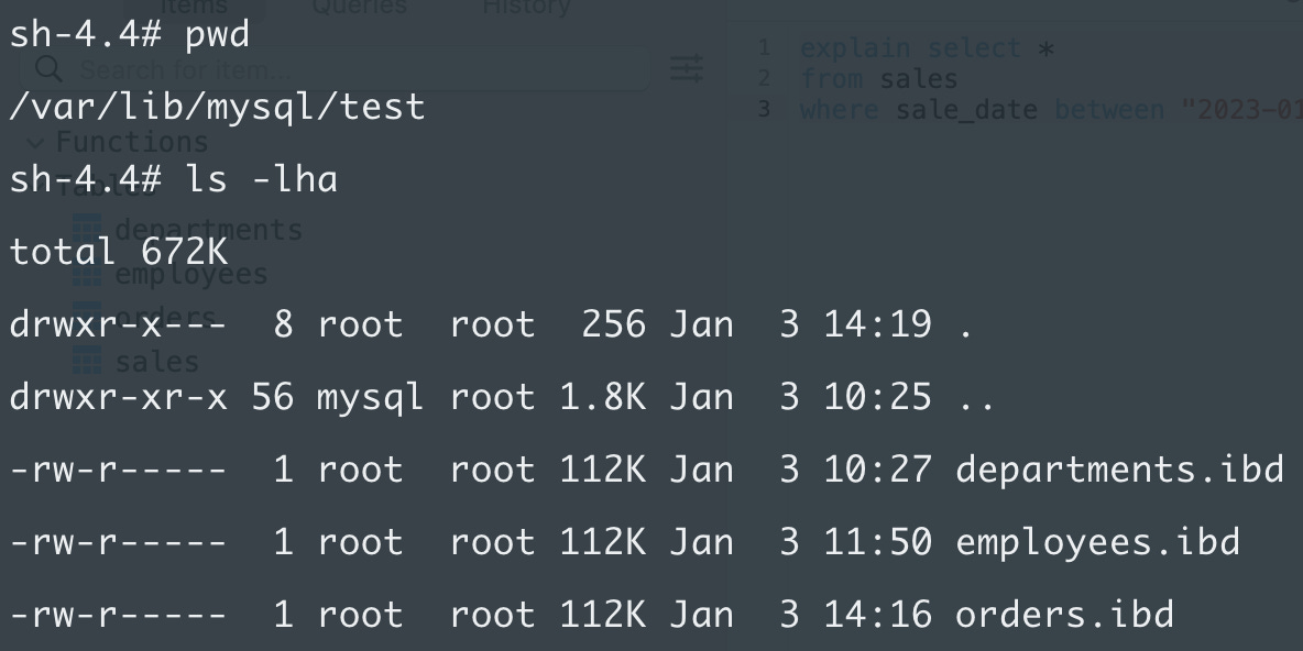
These are just small test tables. Here you can see bigger one:

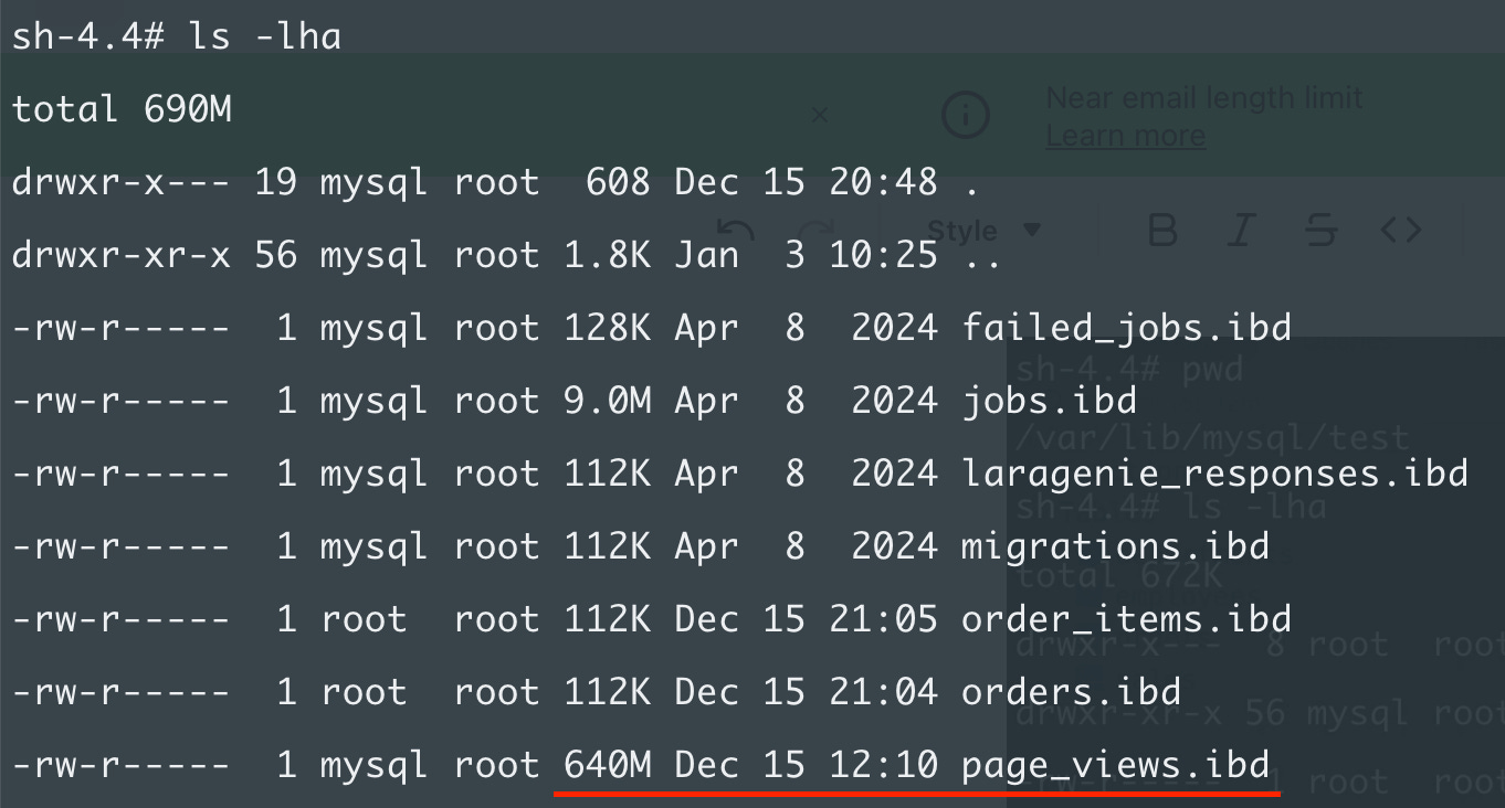
The page_views table is 640MB and it’s not even that big. It contains only a few million rows.

When you run a full table-scan query (or more efficient queries that still need to run I/O operations) MySQL needs to read this 640MB file and look for your records.

Partitioning offers a way to split up these large tables into multiple smaller files.

There are different types of partitioning, for example:

• Range
• List
• Hash

Each of them requires a partition key but they work differently. Let’s look at range. It usually involves a date column, such as created_at. Let’s say, the table contains the following dates:

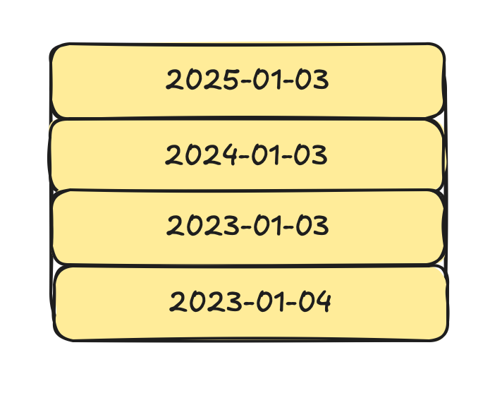
We can create range partitions based on the year, for example. This way, every year has its own partition:

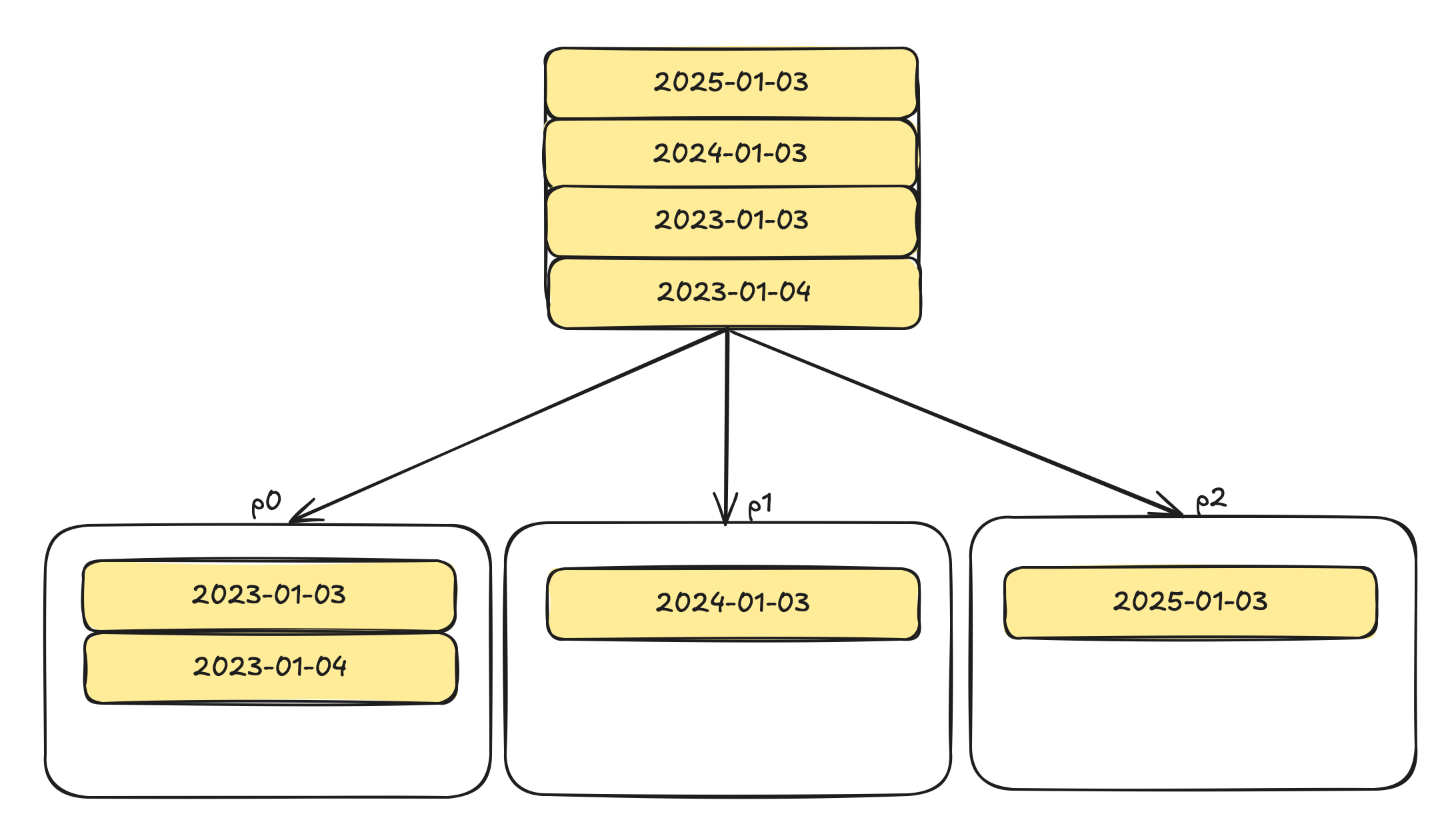
p0, p1, and p2 are arbitrary names for the partitions.

The advantage is that if you have a query like this:

where created_at between "2024-01-01 00:00:00" and "2024-12-31 23:59:59"

MySQL only needs to look at p1 because only p1 contains data from 2024.

If your table has 1 million rows every year, you can serve this query by scanning through only 1 million rows instead of 3 millions. Instead of ~500MB MySQL only needs to read ~160MB. Of course, there are caveats, such as using indexes, not scanning through each row, etc but it’s just an example.

Now, let’s create a table with range partitions based on a date column:

create table orders (
    id bigint not null auto_increment,
    order_date date not null,
    total_amount int not null,
    primary key (id, order_date)
)
partition by range (year(order_date)) (
    partition p0 values less than (2023),
    partition p1 values less than (2024),
    partition p2 values less than MAXVALUE
);

This creates a table with 3 partitions: p0, p1, p2. p0 contains every row where the year is less than 2023. p1 contains rows with a year of 2023 (since it’s less than 2024 but not less than 2023) and then p2 contains everything else.

On the disk, there are now 3 files for the orders table:

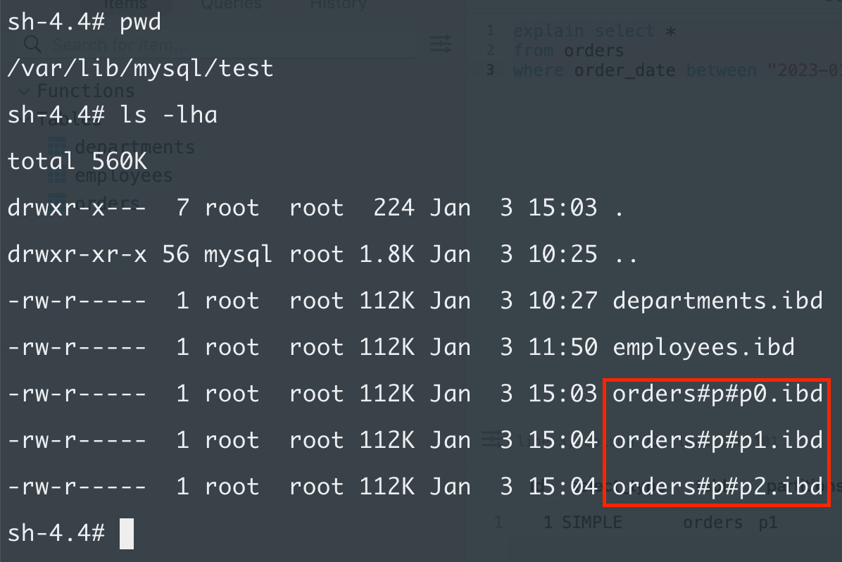
p0, p1, and p2 are part of the filename.

Given the following rows:

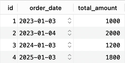
If we run this query:

explain select *
from orders
where order_date between "2023-01-01 00:00:00" and "2023-12-31 23:59:59"

We can see in the explain output that it used only one partition:

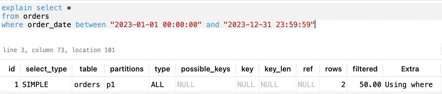
The partitions column says p1 which means MySQL only scanned through the orders#p#p1.ibd file because it contains every record from 2023.

If I extend the range until 2024 the partitions column contains p1 and p2 as well:

That’s because records from 2024 are stored in p2 so now MySQL needs to scan both orders#p#p1.ibd and orders#p#p2.ibd

Partitions are very useful and rarely used in my experience.

There are other types of partitions as well:

LIST. What if you have lots of records in a table, for example every citizen of a country. Each person lives in a city or state. This is a good candidate for a partition. But state names don’t form ranges such as dates. It’s a fixed-length list:

PARTITION BY LIST (state) (
  PARTITION p_northeast VALUES IN ('MA', 'NY', 'CT'),
  PARTITION p_southeast VALUES IN ('FL', 'GA', 'SC')
)

You can partitions your citizens based on their location using list-based partitions. And that has an interesting implication.

A partition is similar to an index.

You want to choose your partition key and type based on the queries you execute. If you mostly query citizens based on their location then having the state column as your key is a good option.

But if you query your table mostly based on the birth_date column (for example) then you’re better off with a range partition.

What if you cannot decide because it’s not that easy?

HASH. In this case, you can use a hash-based partition. It distributes rows evenly across a specified number of partitions based on a user-defined expression:

PARTITION BY HASH (id) PARTITIONS 4

It creates four partitions, and stores your records in them based on the hash representation of the ID column.

There are other types of partitions but I think these are the most important ones. Check out the full list here.

These are three important but somehow less-known MySQL features that you can use in almost any application.

Honorable mentions

• Invisible columns. You can mark columns as “invisible” so they won’t be included in a select * query. This is a great security feature because it decreses the chance of me exposing my users’ passwords. The best candidates for invisible columns are passwords, api keys, and any other auth-related columns.
• Invisible indexes. You can mark an index as invisible as well. The index will remain updated by MySQL but it won’t be used by the query optimizer. It is a great feature if you want to test indexes on big databases because creating a new index or dropping an existing one takes a ong time if you have lots of records.
• JSON columns. This is more well-known I guess, but I still see JSON data being dumped in longtext columns. MySQL has a JSON data type and it offers native support for querying based on keys, for example:

SELECT id, JSON_EXTRACT(data, '$.name') AS name
FROM users
WHERE JSON_EXTRACT(data, '$.age') > 25;

• Full text search. Very important feature and lots of developers use text columns and LIKE % queries instead of a full text index. I wrote about this topic in this article.

Building a database engine

This whole article comes from my book - Building a database engine

It's going to be available on the 8th of April. It discusses topics like:

• Storage layer
• Insert/Update/Delete/Select
• Write Ahead Log (WAL) and fault tolerancy
• B-Tree indexes
• Hash-based full-text indexes
• Page-level caching with LRU
• ...and more

Check it out and pre-order to get the best price: