« back published by Martin Joo on April 23, 2024
Database Indexing in Theory
My goal in this article is to give you the last indexing tutorial you'll ever need.
This is one of the most important topics to understand, in my opinion. No matter what kind of application you're working there's a good chance it has a database. So it's really important to understand what happens under the hood and how indexes actually work. Because of that, this chapter starts with a little bit of theory.
In order to understand indexes, first we need to understand at least 6 data structures:
- Arrays
- Linked lists
- Binary trees
- Binary search trees
- B-Trees
- B+ Trees
Arrays
They are one of the oldest data structures. We all use arrays on a daily basis so I won't go into details, but here are some of their properties from a performance point of view:
| Operation | Time complexity | Space complexity |
|---|---|---|
| Accessing a random element | O(1) | O(1) |
| Searching an element | O(N) | O(1) |
| Inserting at the beginning | O(N) | O(N) |
| Inserting at the end | O(1) or O(N) if the array is full | O(1) |
| Inserting at the middle | O(N) | O(N) |
An array is a fixed sized contiguous data structure. The array itself a pointer to a memory address and each subsequent element has a memory of x + (sizeof(t) * i) where
xis the first memory address where the array points atsizeof(t)is the size of the data type. For example, aninttakes up 8 bytesiis the index of the current element
This is what an array looks like:

The subsequent memory address has an interesting implication: your computer has to shift the elements when inserting or deleting an item. This is why mutating an array in most cases is an O(n) operation.
Since it's a linear data structure with subsequent elements and memory addresses searching an element is also an O(n) operation. You need to loop through all the elements until you find the you need. Of course, you can use binary search if the array is sorted. Binary search is an O(log N) operation and quicksort is an O(N * log N) one. The problem is that you need to sort the array every single time you want to find an element. Or you need to keep it sorted all the time which makes inserts and deletes even worse.
What arrays is really good at is accessing random elements. It's an O(1) operation since all PHP needs to do is calculating the memory address based on the index.
The main takeaway is that searching and mutating is slow.
Linked list
Since arrays have such a bad performance when it comes to inserting and deleting elements engineers came up with linked list to solve these problems.
A linked list is a logical collection of random elements in memory. They are connected only via pointers. Each item has a pointer to the next one. There's another variation called doubly linked list where each element has two pointers: one for the previous and one for the next item.
This is what it looks like:

The memory addresses are not subsequent. This has some interesting implications:
| Operation | Time complexity | Space complexity |
|---|---|---|
| Accessing a random element | O(N) | O(1) |
| Searching an element | O(N) | O(1) |
| Inserting at the beginning | O(1) | O(1) |
| Insertintg at the end | O(1) | O(1) |
| Inserting at the middle | O(N) | O(1) |
Since a linked list is not a coherent structure in memory, inserts always have a better performance compared to an array. PHP doesn't need to shift elements. It only needs to update pointers in nodes.
A linked list is an excellent choice when you need to insert and delete elements frequently. In most cases, it takes considerable less time and memory.
However, searching is as slow as it was with arrays. It's still O(n).
Binary tree
The term binary tree can be misleading since it has lots of special versions. However, a simple binary means a tree where every node has two or less children.
For example, this is a binary tree:
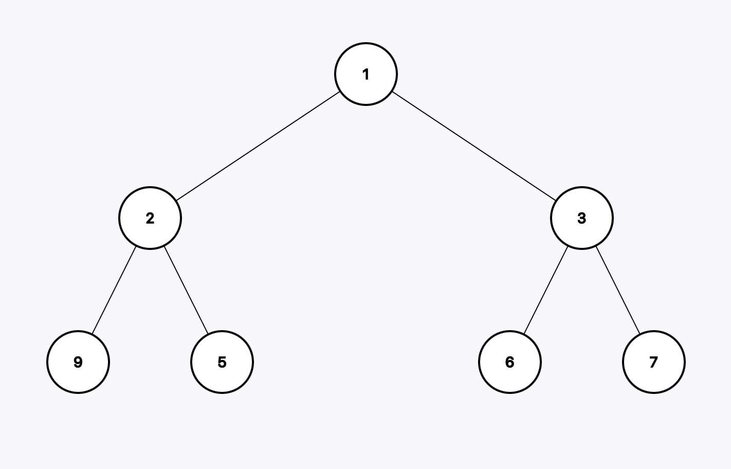 Two only important property of this tree is that each node has two or less children.
This is also a binary tree with the same values:
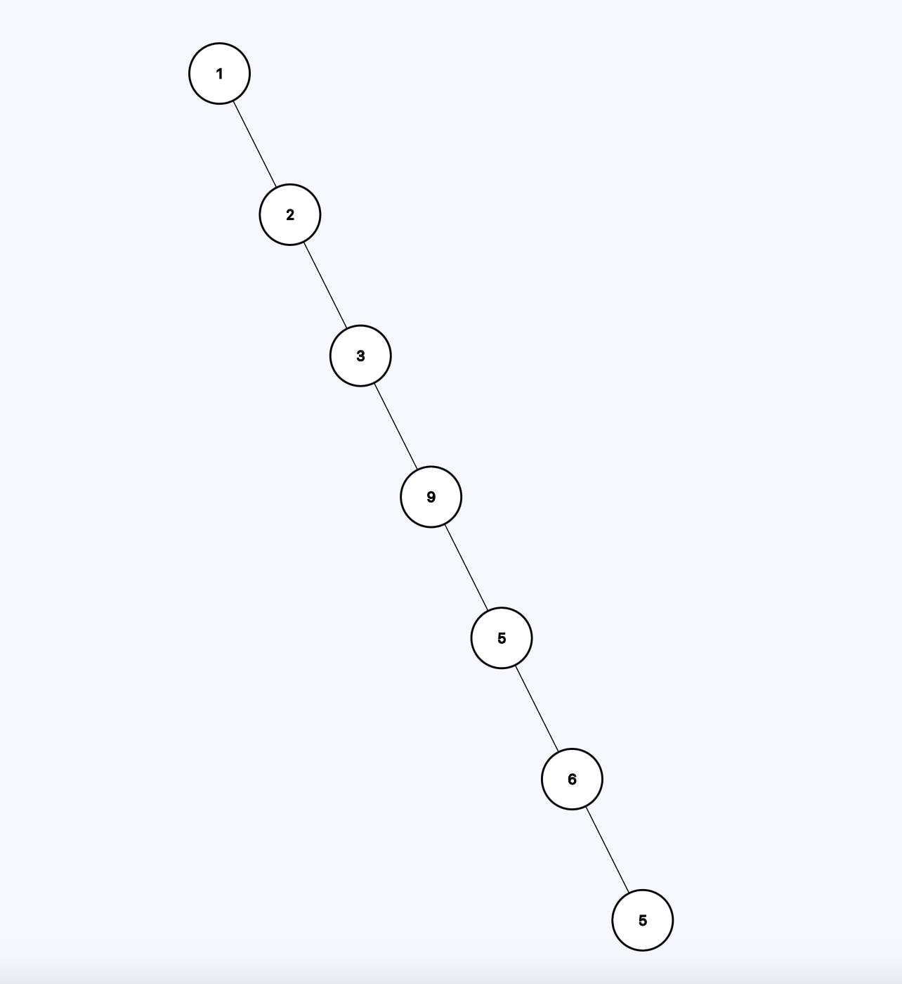
Now, let's think about how much does it take to traverse a binary tree? For example, in the first tree, how many steps does it take to traverse from the root node to one of the leaf nodes (9, 5, 6, 5)? It takes three steps. If I want to go the the left-most node (9) it'd look like (we're already at the root node):
- 2
- 9
Now let's do the same with the second tree. How many steps does it take to go to the leaf node (to 43, strarting from the root)? 6 steps.
Both trees have 7 nodes. Using the first one takes only 2 steps to traverse to one of the leaf node but using the second one takes 6 steps. So the number of steps is not a function of the number of nodes but the height of the tree which is 2 in the first one and 6 in the second one. We don't count the root node.
Both of these trees has a name. The first one is a complete tree meaning every node has exactly two children. The second one is degenerative tree meaning each parent has only one child. These are the two ends of the same spectrum. The first one is perfect and the other one is useless.
In a binary tree, density is the key. The goal is to represent the maximum number of nodes in the smallest depth binary tree possible.
The minimum height of a binary tree is log n which is shown in the first picture. It has 7 elements and the height is 3.
The maximum height possible is n-1 which is shown in the second picture. 7 elements with a height of 6.
From these observations we can conclude that traversing a binary tree is an O(log h) operation where h is the height of the tree.
| # of elements | Height | Time complexity | |
|---|---|---|---|
| Complete tree | 7 | 3 | O(log n) |
| Degenerate tree | 7 | 6 | O(n-1) |
To put it in context, if you have a tree with 100,000,000 elements and your CPU can run 100,000,000 operations per seconds:
| # of iterations | Time to complete | |
|---|---|---|
| O(log n) | 26 | 0,00000026 seconds |
| O(n - 1) | 99,999,999 | 0,99 seconds |
There's a 3,846,153 times difference between the two so engineers came up with the the following conclusion: if a tree is structured well they can traverse it in O(log n) time which is far better than arrays or linked list.
Binary search tree (BST)
So binary trees can have pretty great time complxity when it comes to traversing their nodes. Can we use them to efficiently search elements in O(log n) time?
Enter the binary search tree:
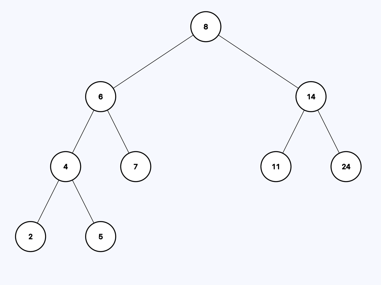
It has three important properties:
- Each node has two or less children
- Each node has a left child that is less than or equal to itself
- Each node has a right child that is greater than itself
The fact that the tree is ordered makes it pretty easy to search elements, for example, this is how we can find 5.
Eight is the starting point. Is it greater than 5? Yes, so we need to continue in the left subtree.
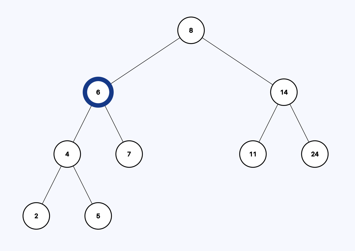
Is 6 greater than 5? Yes, so let's go to the left subtree.
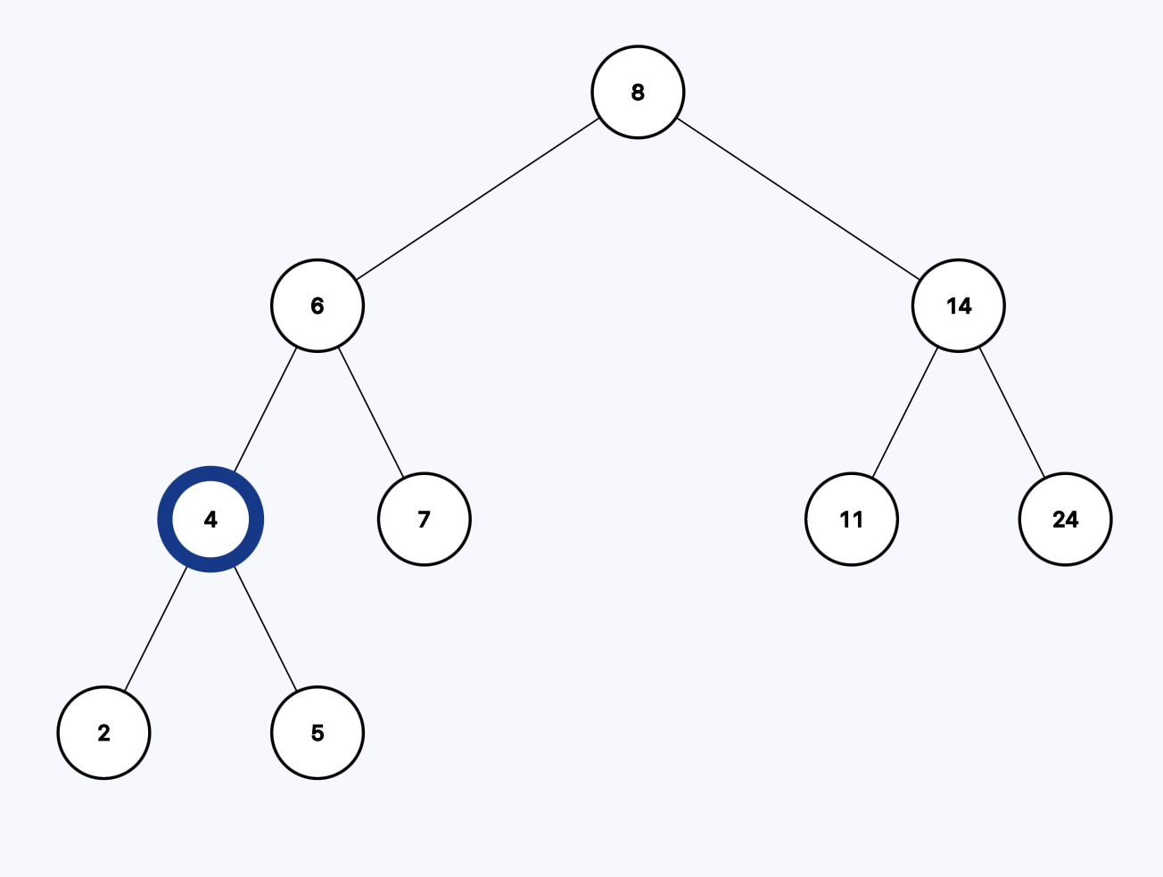
Is 4 greater than 5? Nope. Each node has a right child that is greater than itself. So we go the right.
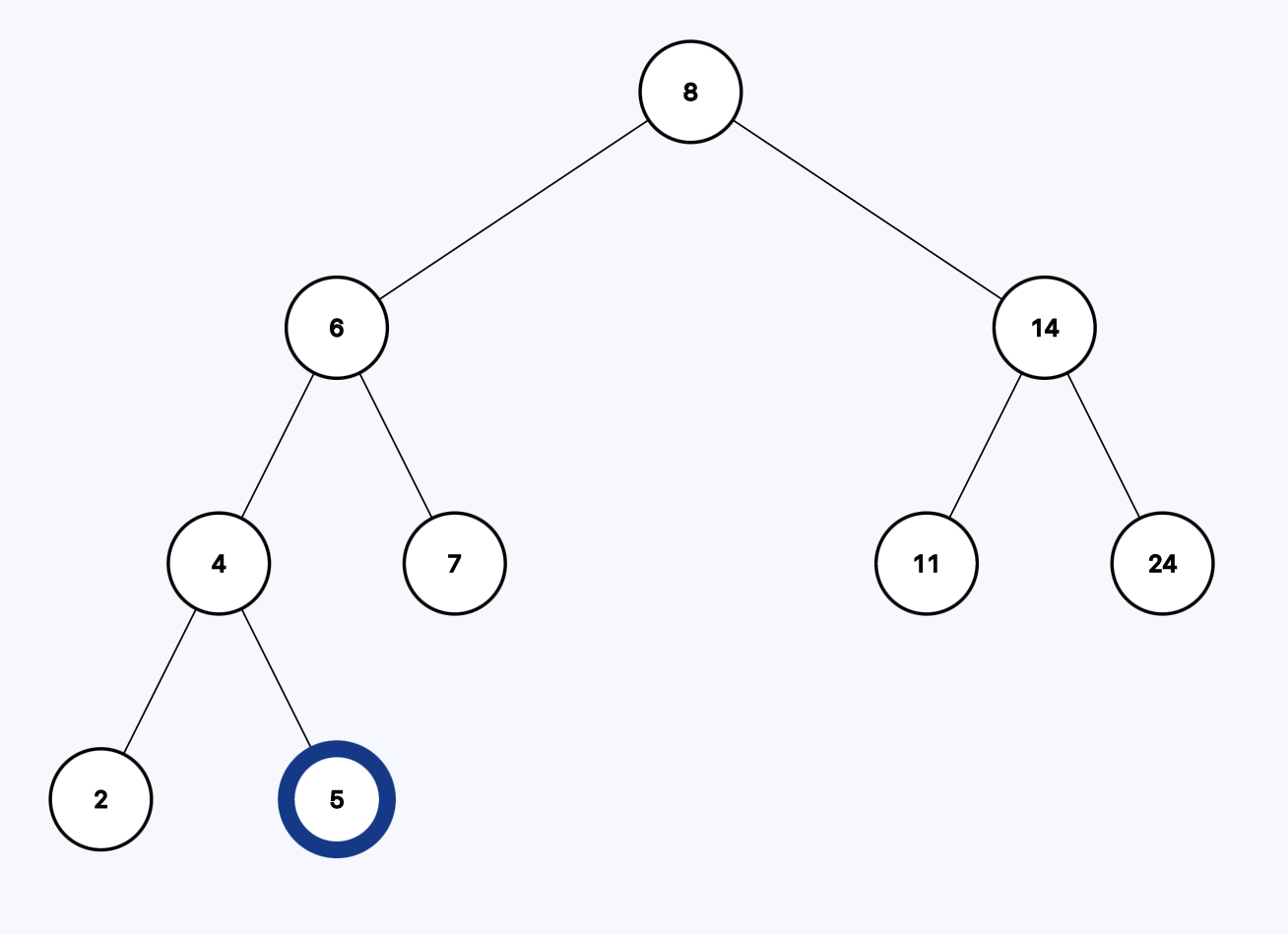
Is 5 equal to to 5? Yes.
We found a leaf node in just 3 steps. The height of the tree is 3, the total number of element is 9. This is the same thing we discussed earlier. The cost of the search is (O log N).
So if we take a usual binary tree and add two constraints to it so it is ordered at any time we have (O log N) search.
Unfortunately, the constraints of a BST don't tell anything about balance. So this is also a perfectly fine BST:
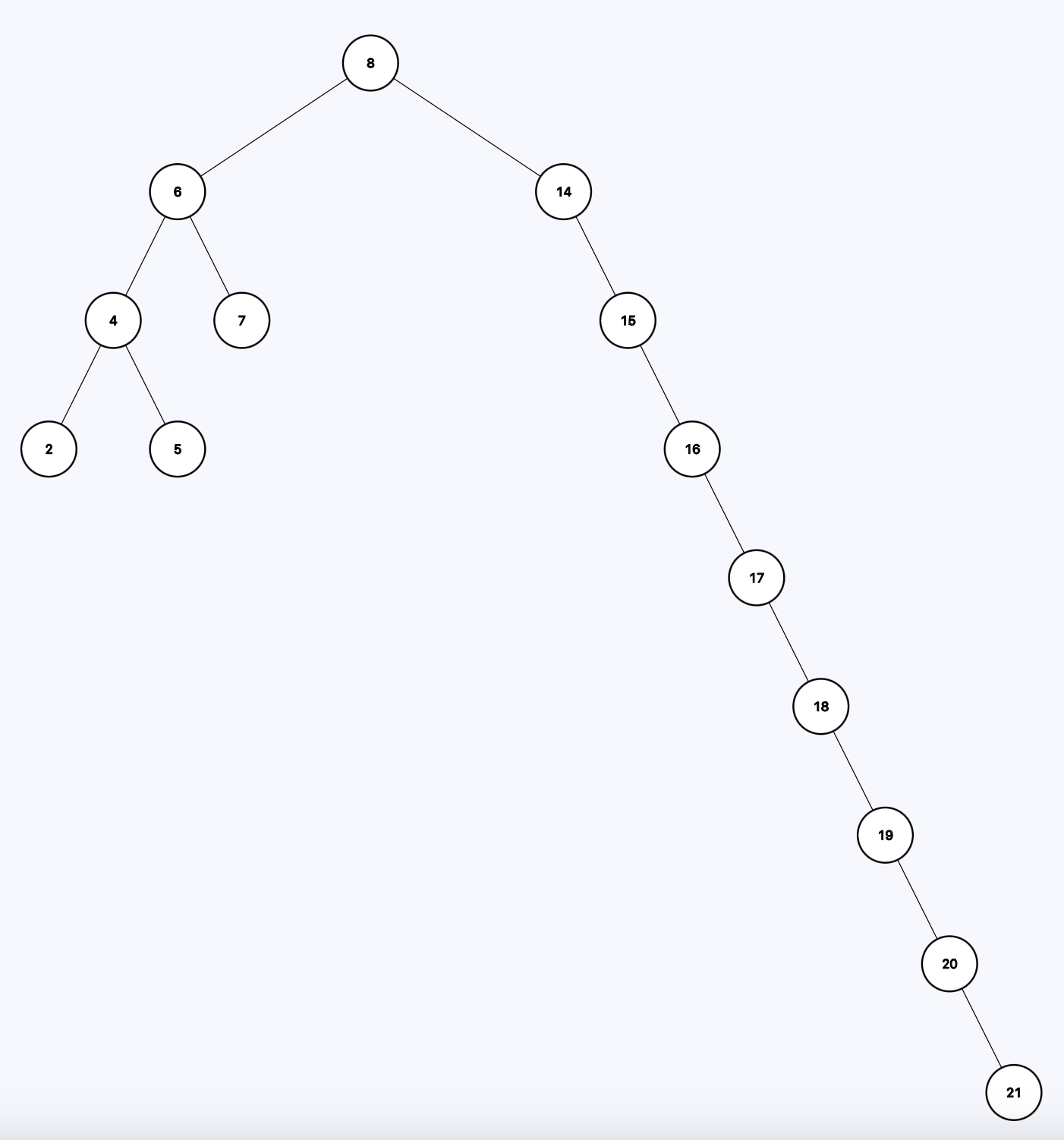
Each node has two or less children. The left child is always less than or equal to the parent. The right child is always greater than the parent. But the right side of the tree is very unbalanced. If you want to find the number 21 (the bottom node in the right subtree) it becomes an O(N) operation.
Binary search trees were invented in 1960, 35 years before MySQL.
Indexing in the early days
Databases and storage systems were emerging in the 1960's. The main problem was the same as today: accessing data was slow because of I/O operations.
Let's say we have a really simple users table with 4 columns:
| ID | name | date_of_birth | job_title |
|---|---|---|---|
| 1 | John Doe | 2005-05-15 | Senior HTML programmer |
| 2 | Jane Doe | 1983-08-09 | CSS programmer |
| 3 | Joe Doe | 1988-12-23 | SQL programmer |
| 4 | James Hetfield | 1969-08-03 | plumber |
For simplicity, let's assume a row takes 128 bytes to store on the disk. When you read something from the disk the smallest unit possible is 1 block. You cannot just randomly read 1 bit of information. The OS will return the whole block. For this example, we assume a block is 512 bytes. So we can fit 4 records (4 * 128B) into one block (512B). If we have 100 records we need 25 blocks.
| Size of a record | 128B |
| Size of a block | 512B |
| # of records in one block | 4 |
| # of records overall | 100 |
| # of block needed to store the table | 25 |
If you run the following query against this table (assuming no index, no PK):
select *
from users
where id = 50
Something like this happens:
- The database will loop through the table
- It reads the first block from disk that contains row #1 - row #4
- It doesn't contain user #50 so it continues
In the worst-case scenario, it executes 25 I/O operations scanning the table block-by-block. This is called a full table scan. It's slow. So engineers invented indexing.
Single-level indexing
As you can see, the problem was the size and the number of I/O operations. Can we reduce it by introducing some kind of index? Some kind of secondary table that is smaller and helps reduce I/O operations? Yes, we can.
Here's a simple index table:
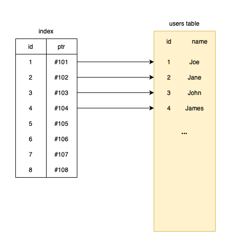
The index table stores every record that can be found in users. They both have 100 rows. The main benefit is that the index is small. It only holds an ID that is equivalent to the ID in the users table and a pointer. This pointer points to the row on the disk. It's some kind of internal value with a block address or something like that. How big is this index table?
Let's assume that both the ID and ptr columns take up 8 bytes of space. So a record's size in the index table is 16 bytes.
| Size of a record | 16B |
| Size of a block | 512B |
| # of records in one block | 32 |
| # of records overall | 100 |
| # of blocks needed to store the index table | 4 |
Only 4 blocks are needed to store the entire index on disk. To store the entire table the number of blocks is 25. It's a 6x difference.
Now what happens when we run?
select *
from users
where id = 50
- The database reads the index from the disk block-by-block
- It means 4 I/O operations in the worst-case scenario
- When it finds #50 in the index it queries the table based on the pointer which is another I/O
In the worst-case scenario, it executes 5 I/O operations. Without the index table, it was 25. It's a 5x performance improvement. Just by introducing a "secondary table."
Multi-level indexing
An index table made things much better, however, the main issue remained the same: size and I/O operations. Now, imagine that the original users table contains 1,000 records instead of 100. This is what the I/O numbers would look like:
| # of blocks to store the data | # of I/O to query data | |
|---|---|---|
| Database table with 1,000 users | 250 | 250 |
| Index table with 1,000 users | 40 | 41 |
Everything is 10x larger, of course. So engineers tried to divide the problem even more by chunking the size into smaller pieces and they invented multi-level indexes. Now we said that you can store 32 entries from the index table in a single block. What if we can have a new index where every entry points to an entire block in the index table?
Well, this is a multi-level index:
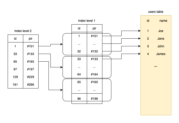
Each entry in the second level index points to a range of records in the first level index:
-
Row #1 in L2 points to row #1 - row #32 in L1
-
Row #2 points to row #33 - row #64
-
etc
Each row in L2 points to a chunk of 32 rows in L1 because that's how many records can fit into one block of disk.
If the L1 index can be stored using 40 blocks (as discussed earlier), then L2 can be stored using 40/32 blocks. It's because in L2 every record points to a chunk of 32 records in L1. So L1 is 32x bigger than L2. 1,000 rows in L1 is 32 rows in L2.
The space requirement for L2 is 40/32 or 2 blocks.
| # of blocks to store the data | |
|---|---|
| Database table with 1,000 users | 250 |
| L1 index with 1,000 users | 40 |
| L2 index with 1,000 users | 2 |
What happens when we run:
select *
from users
where id = 50
- The database reads L2 block-by-block
- In the worst-case scenario, it read 2 blocks from the disk
- It finds the one that contains user #50
- It reads 1 block from L1 that contains user #50
- It reads 1 block from the table that contains user #50
Now we can find a specific row by just reading 4 blocks from the disk.
| # of blocks to store the data | # of I/O to query data | |
|---|---|---|
| Database table with 1,000 users | 250 | 250 |
| L1 index with 1,000 users | 40 | 41 |
| L2 index with 1,000 users | 2 | 4 |
They were able to achieve a 62x performance improvement by introducing another layer.
Now let's do something crazy. Rotate the image by 90 degrees:
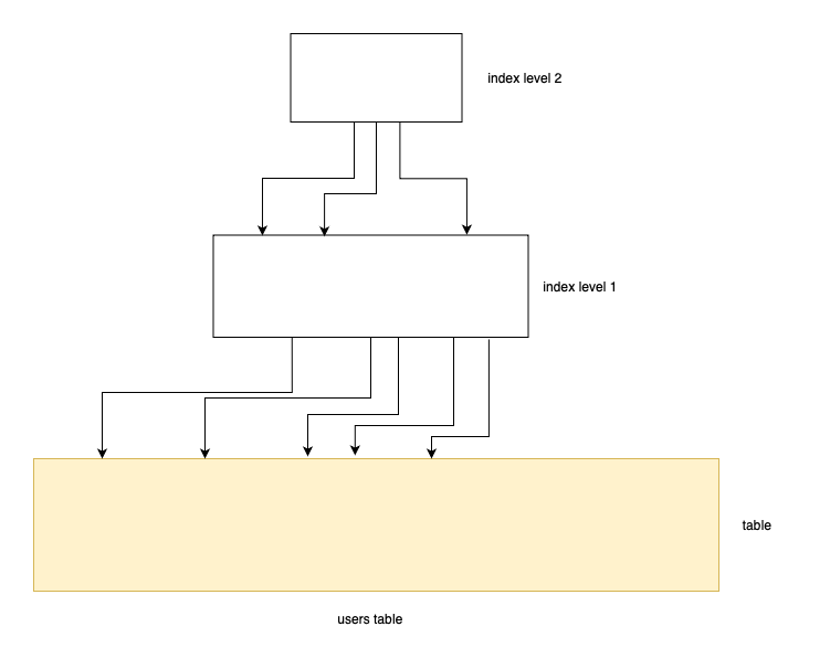
It's a tree! IT'S A TREE!!
B-Tree
In 1970, two gentlemen at Boeing invented B-Trees which was a game-changer in databases. This is the era when Unix timestamps looked like this: 1 If you wanted to query the first quarter's sales, you would write this: between 0 and 7775999. Black Sabbath released Paranoid. Good times.
What does the B stand for? They didn't specify it, but often people call them "balanced" trees.
A B-Tree is a specialized version of an M-way tree. "What's an M-way tree?" Glad you asked!
This is a 3-way tree:
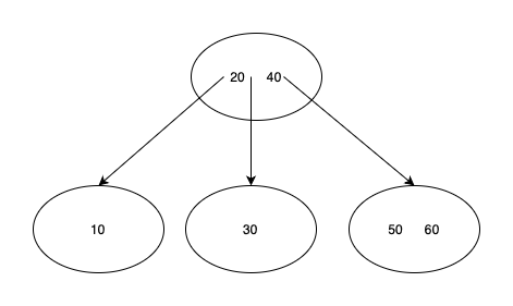
It's a bit different than a binary tree:
- Each node holds more than one value. To be precise a node can have m-1 values (or keys).
- Each node can have up to m children.
- The keys in each node are in ascending order.
- The keys in children nodes are also ordered compared to the parent node (such as 10 is at the left side of 20 and 30 is at the right side)
Since it's a 3-way tree a node can have a maximum of 3 children and can hold up to two values.
If we zoom in on a node it looks like this:
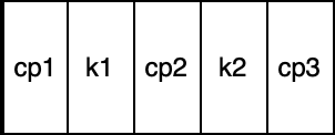
cp stands for child pointer and k stands for key.
The problem is however, there are no rules or constraints for insertion or deletion. This means you can do whatever you want, and m-way trees can become unbalanced just as we see with binary search trees. If a tree is unbalanced searching becomes O(n) which is very bad for databases.
So B-Trees are an extension of m-way search trees. They define the following constraints:
- The root node has at least 2 children (or subtrees).
- Each other node needs to have at least m/2 children.
- All leaf nodes are at the same level
I don't know how someone can be that smart but these three simple rules make B-trees always at least half full, have few levels, and remain perfectly balanced.
There's a B-Tree visualizer website where you can see how insertion and deletion are handled and how the tree remains perfectly balanced at all times.
Here you can see numbers from 1 to 15 in a 4-degree B-Tree:
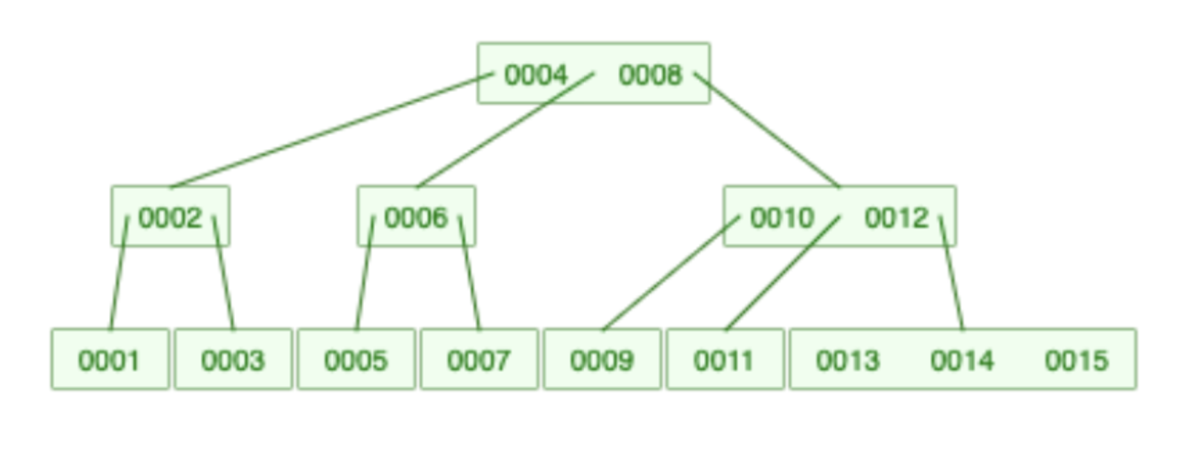
Of course, in the case of a database, every node has a pointer to the actual record on disk just as we discussed earlier.
The next important thing is this: MySQL does not use a standard B-Tree. Even though we use the word BTREE when creating an index it's actually a B+ Tree. It is stated in the documentation:
The use of the term B-tree is intended as a reference to the general class of index design. B-tree structures used by MySQL storage engines may be regarded as variants due to sophistications not present in a classic B-tree design. - MySQL Docs
It is also said by Jeremy Cole multiple times:
InnoDB uses a B+Tree structure for its indexes. - Jeremy Cole
He built multiple forks of MySQL, for example, Twitter MySQL, he was the head of Cloud SQL at Google and worked on the internals of MySQL and InnoDB.
Problems with B-Trees
There are two issues with a B-Tree. Imagine a query such as this one:
select *
from users
where id in (1,2,3,4,5)
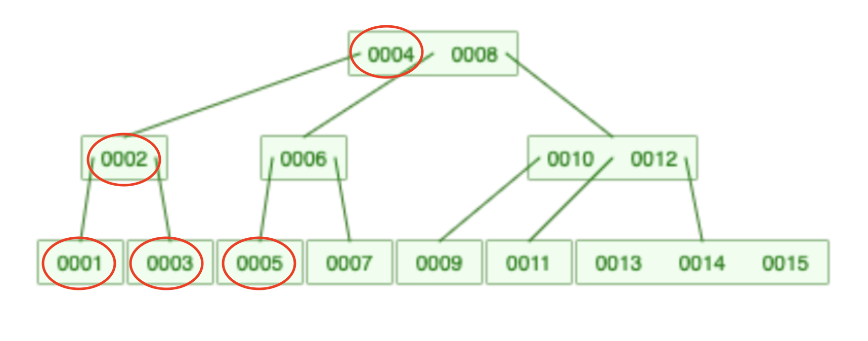
It takes at least 8 steps to find these 5 values:
- From 4 to 2
- From 2 to 1
- From 1 back to 2
- From 2 to 3
- From 3 to 2
- From 2 to 4
- From 4 to 6
- From 6 to 5
So a B-Tree is not the best choice for range queries.
The other problem is wasting space. There's one thing I didn't mention so far. In this example, only the ID is present on the tree. Because this example is a primary key index. But of course, in real life, we add indexes to other columns such as usernames, created_at, other dates, and so on. These values are also stored in the tree.
An index has the same number of elements as the table so the size of it can be huge if the table is big enough. This makes a B-Tree less optimal to load into memory.
B+ Trees
As the available size of the memory grew in servers, developers wanted to load the index into memory to achieve really good performance. B-Trees are amazing, but as we discussed they have two problems: size and range queries.
Surprisingly enough, one simple property of a B-Tree can lead us to a solution: most nodes are leaf nodes. The tree above contains 15 nodes and 9 of them are leaves. This is 60%.
Sometime around 1973, someone probably at IBM came up with the idea of a B+ Tree:

This tree contains the same numbers from 1 to 15. But it's considerably bigger than the previous B-Tree, right?
There are two important changes compared to a B-Tree:
- Every value is present as a leaf node. At the bottom of the tree, you can see every value from 1 to 15
- Some nodes are duplicated. For example, number 2 is present twice on the left side. Every node that is not a leaf node in a B-Tree is duplicated in a B+ Tree (since they are also inserted as leaf nodes)
- Leaf nodes form a linked list. This is why you can see arrows between them.
- Every non-leaf node is considered as a "routing" node.
With the linked list, the range query problem is solved. Given the same query:
select *
from users
where id in (1,2,3,4,5)
This is what the process looks like:

Once you have found the first leaf node, you can traverse the linked list since it's ordered. Now, in this specific example, the number of operations is the same as before, but in real life, we don't have a tree of 15 but instead 150,000 elements. In these cases, linked list traversal is way better.
So the range query problem is solved. But how does an even bigger tree help reduce the size?
The trick is that routing nodes do not contain values. They don't hold the usernames, the timestamps, etc. They are routing nodes. They only contain pointers so they are really small items. All the data is stored at the bottom level. Only leaf nodes contain our data.
Leaf nodes are not loaded into memory but only routing nodes. As weird as it sounds at first according to PostgreSQL this way the routing nodes take up only 1% of the overall size of the tree. Leaf nodes are the remaining 99%:
Each internal page (comment: they are the routing nodes) contains tuples (comment: MySQL stores pointers to rows) that point to the next level down in the tree. Typically, over 99% of all pages are leaf pages. - PostgreSQL Docs
So database engines typically only keep the routing nodes in memory. They can travel to find the necessary leaf nodes that contain the actual data. If the query doesn't need other columns it's essentially can be served using only the index. If the query needs other columns as well, MySQL reads it from the disk using the pointers in the leaf node.
I know this was a long introduction but in my opinion, this is the bare minimum we should know about indexes. Here are some closing thoughts:
- Both B-Trees and B+ trees have
O(log n)time complexity for search, insert, and delete but as we've seen range queries perform better in a B+ tree. - MySQL (and Postgres) uses B+ Trees, not B-Trees.
- The nodes in real indexes do not contain 3 or 4 keys as in these examples. They contain thousands of them. To be precise, a node matches the page size in your OS. This is a standard practice in databases. Here you can see in MySQL's source code documentation that the
btr_get_sizefunction, for example, returns the size of the index expressed as the number of pages.btr_stands forbtree. - Interestingly enough MongoDB uses B-Trees instead of B+ Trees as stated in the documentation. Probably this is why Discord moved to Cassandra. They wrote this on their blog:
Around November 2015, we reached 100 million stored messages and at this time we started to see the expected issues appearing: the data and the index could no longer fit in RAM and latencies started to become unpredictable. It was time to migrate to a database more suited to the task. - Discord Blog
All of these examples come from my new book Performance with Laravel. There's a 60-page chapter in the book dedicated only to database indexing. This article is the introduction to the chapter.
Check it out:
